January 17, 2026
Machine Learning Classification


Classification is one of the most common tasks in machine learning. It covers a wide variety of business needs from predicting player’s churn in mobile gaming to fraud detection in banking. Although each problem demands a specific approach and deep business understanding, it is still possible to extract common patterns that appear while approaching all these problems with machine learning. This article will cover some of them and if you want to read about some basics please go to Machine Learning Basics.
Key Takeaways
- Classification is a supervised ML task where a model learns to assign each input to one of a fixed set of categories — used in fraud detection, churn prediction, image recognition, sentiment analysis and many more.
- There are four main types: binary (two classes), multi-class (one of many), multi-label (multiple at once), and imbalanced (one class is rare).
- The most common algorithms are logistic regression, gradient boosting (XGBoost, LightGBM), and — for unstructured data — deep learning. Gradient boosting wins most tabular classification problems in industry today.
- Accuracy is rarely the right metric. For imbalanced or asymmetric-cost problems, use precision, recall, F1-score or PR-AUC depending on what’s actually costly when the model is wrong.
- The hard work in classification is usually data preparation, class definition, and metric selection — not picking the algorithm.
Machine Learning classification – High-level overview
In simple words, classification is a machine learning task in which the model is taught to distinguish things (items, users, transactions, etc.) between two (binary classification) or more (multiclass classification) classes. As an example, consider churn prediction in gaming – all active users are classified either as low-churn-risk (first class) or high-churn-risk (second class). This allows us to approach those two groups of gamers with different means (ads, offers) and by this encourage more players to keep playing the game – at the same time increasing the company’s ROI from players’ payments or in-game ads.
To simplify, we will use the gaming example throughout this article. Keep in mind that the problems we will discuss are much more general and appear in almost all classification tasks.
Types of Machine Learning Classification
Classification problems differ in how many classes are involved and how those classes relate to each individual example. There are four main types you’ll encounter:
Binary classification
The simplest case — each example belongs to exactly one of two classes. Examples: spam vs not-spam, fraud vs legitimate transaction, churn vs retain, disease present vs absent. Most real-world business classification problems start here.
Multi-class classification
Each example belongs to exactly one of three or more classes. Examples: classifying news articles into topics (politics, sport, business, technology), recognizing handwritten digits 0–9, predicting which product category a customer will buy next. The classes are mutually exclusive — a single news article can only be in one category.
Multi-label classification
Each example can belong to multiple classes at the same time. Examples: tagging a movie as both “comedy” and “romance,” detecting all the objects visible in a photo, assigning multiple medical conditions to a patient record. The model outputs a set of labels, not a single one.
Imbalanced classification
A binary or multi-class problem where one class is dramatically more common than the others — fraud detection (typically <1% positive cases), rare disease screening, equipment failure prediction. These problems are technically the same as standard classification but need different metrics and often specialized techniques (resampling, class weighting, anomaly detection).
Identifying which type your problem belongs to is one of the first decisions in any classification project — it shapes both model choice and which metrics matter.
What kind of answer would you like to get from Machine Learning classification?
In the simplest case, when using the machine learning model to make predictions, it can return the label of a class it thinks that the given example belongs to. So in our example, it would correspond to informing if each user is most likely to churn or not churn. An alternative approach is to return the estimated probability of belonging to each class, e.g. for a given user the model would predict 95% of churn and 5% of staying in-game.
How to prepare data for Machine Learning?
Most models accept only numerical features. This means that what you need to do before feeding data to the model is to clean it. There might be many things to do, let us list some of them:
- Fill missing values. Some models accept missing (unknown) values, some do not. To fill those gaps in data, first, you should understand their origin – maybe missing data contains some information? Maybe there is an obvious interpretation of it and it can be replaced with the number corresponding to that interpretation? Maybe data is simply corrupted?
- Standardize features. Some models require features to be of the same magnitude to learn effectively. The simplest approach is to subtract the mean from each feature value and divide it by its standard deviation.
- Encode categorical features. Categorical features (e.g. person’s sex) should be encoded with numbers. Moreover, if there are more than two possible values, they should be encoded into binary variables (e.g. sex could be encoded as binary variables: sex_male, sex_female, sex_other). This procedure is known as one-hot encoding.

Dataset
We will use the titanic dataset as it is simple and contains both continuous and categorical columns.


Machine Learning models
There’s no single “best” classification algorithm — the right choice depends on your data, the number of features, the size of your dataset, and the trade-off between accuracy and interpretability. Here are the algorithms data scientists reach for most often:
- Logistic Regression — Despite the name, it’s a classification algorithm. Fast, interpretable, and a strong baseline. Best for linear relationships and when you need to explain why the model made a decision (regulated industries, credit scoring).
- Decision Trees — Easy to visualize and interpret. They split data into yes/no questions until each branch lands on a class. Prone to overfitting on their own, so usually used as a building block for ensembles.
- Random Forest — An ensemble of many decision trees. Robust, handles missing data well, and works out of the box on most tabular problems. Often the first “real” model data scientists try after logistic regression.
- Gradient Boosting (XGBoost, LightGBM, CatBoost) — Builds trees sequentially, each correcting the previous one’s mistakes. Currently the dominant approach for tabular data in industry and ML competitions. More accurate than random forest, but harder to tune.
- Support Vector Machines (SVM) — Find the optimal boundary between classes. Effective on smaller datasets with many features (e.g., text classification), but slower on very large datasets.
- K-Nearest Neighbors (KNN) — Classifies a new point by looking at its k closest neighbors and taking a vote. Simple and intuitive, but doesn’t scale well to large datasets or many features.
- Naive Bayes — Probabilistic classifier based on Bayes’ theorem. Fast, works well for text classification (spam, sentiment) even with limited training data.
- Neural Networks and Deep Learning — For unstructured data like images, audio, and text, deep learning (CNNs, transformers) outperforms classical methods. For tabular business data, gradient boosting usually still wins.
A practical rule of thumb: start with logistic regression as a baseline, then try gradient boosting (XGBoost or LightGBM) — these two cover 80% of real-world classification problems. Reach for deep learning when your data is unstructured (images, text, audio) or genuinely massive.
Training


Choosing the best model for Machine Learning classification
The first will be used to pick the best model and the second to validate it. This way we make sure that the metrics we evaluate on the test set will correspond to the ones measured when the model is applied in production.
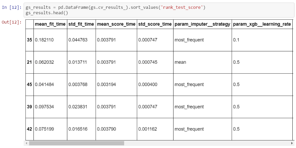
Then, to choose the best model and its hyperparameters we perform so-called grid search (or one of its alternatives e.g. Bayes optimization). Grid search consists of two parts:
- fitting every possible parameter set from specified lists and evaluating results it gives,
- cross-validation – the model is being fitted as a part of the training set and then evaluated on the remaining part. This process is repeated a given number of times for each parameter combination.
This approach is much more time consuming than a simple train-test but gives us higher confidence about the quality of the final model.
Real-world classification use cases
Classification is one of the most widely deployed ML techniques in production. A few representative examples:
- Finance — fraud detection. Each card transaction is classified as legitimate or fraudulent in real time, typically using gradient boosting models combined with rule-based safeguards. The class imbalance is extreme (<0.1% positives), which drives the choice of metrics (precision-recall AUC, not accuracy).
- Healthcare — disease screening. Medical images (X-rays, MRIs, retinal scans) are classified as showing a particular condition or not. Deep learning (convolutional neural networks) dominates here. Misclassification costs differ enormously between false positives and false negatives, which shapes the optimization target.
- Marketing — customer churn prediction. Active customers are classified as low or high churn risk so retention offers can be targeted. Usually built on tabular CRM data with gradient boosting.
- Manufacturing — defect detection. Products on a production line are classified as pass or fail using computer vision. Often combined with anomaly detection because defect types evolve over time.
- HR — resume screening. Candidate profiles are classified by likely fit for a role. This is also one of the highest-risk classification applications from a fairness and regulatory standpoint, requiring careful bias auditing.
- NLP — sentiment analysis and intent detection. Customer messages, reviews, or support tickets are classified by sentiment (positive/negative/neutral) or intent (refund request, billing question, complaint). Increasingly built on fine-tuned language models rather than classical algorithms.
What these have in common is that the model is rarely the hardest part. Defining the classes correctly, sourcing labeled data, and choosing the right success metric usually take longer than picking the algorithm.
Metrics
Proper metric choice is crucial for the real-world application of machine learning. It allows us to tell how good the model is and decide whether one model is better than the other. It also makes progress possible – one can track the value of the metric from one experiment to the other and finally choose the configuration with the highest score. Properly adjusted metric also tells how well the business needs are met by the machine learning solution.
Because of numerous metrics that can fit different tasks, we will further limit ourselves to metrics that apply only to binary classification and model returning dichotomous answers.
One of the simplest metrics is accuracy – by definition, it is a percentage of cases in which the model is correct – that clear interpretation is a great advantage from the business perspective. This metric suits well when trying to build a general classification model on the balanced dataset (meaning that the number of each class is approximately the same). It fails however in case of significant class imbalance – consider data in which only 1% of users churn. One can easily reach an accuracy of 99% just by assigning not churn label to each input. In that case, we end up with 99% accuracy and a completely useless model.
| Metric | What it measures | When to use it |
|---|---|---|
| Accuracy | % of correct predictions overall | Balanced classes, no strong cost asymmetry |
| Precision | Of items predicted positive, how many really are positive | When false positives are costly (spam filters, fraud alerts that trigger account freezes) |
| Recall (sensitivity) | Of all real positives, how many were caught | When false negatives are costly (cancer screening, security threat detection) |
| F1-score | Harmonic mean of precision and recall | Imbalanced data; when you care about both precision and recall |
| ROC-AUC | How well the model separates classes across all thresholds | Comparing models; threshold-independent evaluation |
| PR-AUC | Like ROC-AUC but for imbalanced data | Highly imbalanced problems (fraud, rare disease) |
| Log loss | Penalizes confident wrong predictions | When you need calibrated probability outputs |
| Confusion matrix | Full breakdown of true/false positives and negatives | Diagnosing exactly how a model fails |
Two more concepts you’ll meet constantly in classification work:
- ROC-AUC measures how well a model separates classes across every possible probability threshold — from “everything is positive” to “nothing is positive.” A value of 0.5 is random guessing, 1.0 is perfect separation. It’s useful for comparing models without picking a specific threshold yet.
- The confusion matrix is the diagnostic tool behind every other metric — a simple 2×2 (for binary) or N×N table showing true positives, false positives, true negatives, and false negatives. Most metrics above are just different summaries of this same matrix. When a model underperforms, the confusion matrix usually tells you exactly which class is being mis-classified and how.
The most important point about metrics: the right one depends on what’s costly in your specific business problem. A 99% accurate medical screening model that misses every actual cancer is useless. A fraud detector that flags 50% of legitimate transactions costs more in customer churn than it saves in fraud. Choose the metric that reflects the real cost of being wrong.
In the case of imbalanced data, usually, the more complicated metrics are being used. One of them is an f-score which is the harmonic mean of precision (rate of cases in which, while labeling an example by positive class, the model is correct) and recall (detection rate for positive class). Usage of harmonic instead of arithmetic means ensures that to maximize f-score one needs to maximize both precision and recall at the same time, which solves the possible problem of one of them being very low and the other very high.
Depending on the business problems, one may care more about recall than precision, e.g. when detecting customer churn it may be beneficial to pay the price of more players erroneously considered churns (lower precision), in return correctly classifying more players as churns (higher recall). In that case, the f-beta-score function family can be helpful. It is simply f-score with more weight assigned to precision or recall depending on the beta value.
Model evaluation

Summary
Classification is one of the most practical and most widely deployed machine learning techniques — sitting behind fraud detection, medical screening, churn prediction, defect detection, and countless other production systems. The hard part is rarely the algorithm itself: it’s defining the classes correctly, sourcing clean labeled data, choosing the right metric for the business cost of being wrong, and validating that the model generalizes to new data.
A practical workflow looks like this:
- Define the type of classification you’re solving (binary, multi-class, multi-label, imbalanced).
- Prepare your data — cleaning, encoding, handling missing values.
- Start with a simple baseline (logistic regression).
- Try more powerful models (gradient boosting; deep learning if your data is unstructured).
- Use cross-validation and grid search to tune hyperparameters.
- Evaluate with the right metric for your problem — not just accuracy.
- Validate on truly unseen data before deploying.
If you’d like help applying classification to a real business problem — fraud, churn, defect detection, or anything else — book a 30-minute call with our team. We’ll help you map the problem to the right approach.
FAQ
What is classification in machine learning?


Classification is a supervised machine learning task where a model learns to assign each input example to one of a fixed set of categories — for example, marking an email as spam or not spam, or labeling a tumor image as malignant or benign. The model learns from examples whose correct categories are already known, then makes predictions on new, unseen data.
What is the difference between classification and regression?
Both are supervised learning tasks, but they predict different things. Classification predicts a discrete category (spam / not spam, dog / cat / horse). Regression predicts a continuous numerical value (house price, temperature, expected revenue). The same algorithm family — like decision trees or neural networks — can usually do both, with small architectural changes.
What is the difference between binary, multi-class, and multi-label classification?
Binary classification has exactly two possible classes per example (spam / not spam). Multi-class has three or more, but each example belongs to only one (digit recognition: 0–9). Multi-label allows multiple classes for the same example at once (a single movie can be both “comedy” and “romance”).
Which classification algorithm should I use?
Start with logistic regression as a baseline — it’s fast and interpretable. Then try gradient boosting (XGBoost, LightGBM, or CatBoost) — it wins most tabular classification problems in industry today. For unstructured data like images, text, or audio, reach for deep learning (CNNs for images, transformers for text). A practical sequence of “logistic regression → gradient boosting → deep learning if needed” handles the vast majority of business problems.
What does accuracy mean in machine learning classification?
Accuracy is the percentage of predictions that the model gets correct. It’s easy to interpret but can be misleading on imbalanced datasets — if 99% of transactions are legitimate, a model that simply predicts “legitimate” every time is 99% accurate and completely useless. For imbalanced problems, precision, recall, F1-score, or PR-AUC are more informative.
What is overfitting in classification, and how do I prevent it?
Overfitting happens when a model learns the training data so closely — including its noise and quirks — that it fails to generalize to new data. You spot it when training accuracy is much higher than test accuracy. Prevent it with cross-validation, regularization (L1/L2), simpler models, more training data, or early stopping for neural networks.
How much data do I need to train a classification model?
It depends on the algorithm and the problem complexity. Logistic regression can give useful results with a few hundred examples per class. Gradient boosting typically needs at least a few thousand. Deep learning usually needs tens of thousands or more, unless you’re fine-tuning a pre-trained model — in which case a few hundred well-chosen examples can be enough.
Can large language models (LLMs) be used for classification?
Yes — and increasingly often. LLMs can classify text either in a zero-shot way (just describing the categories in the prompt) or after lightweight fine-tuning. For high-volume production use, a fine-tuned smaller model is usually cheaper and faster; for prototyping or low-volume tasks, calling an LLM API directly is often the fastest path.
Category: